Bioacoustic Research Methods

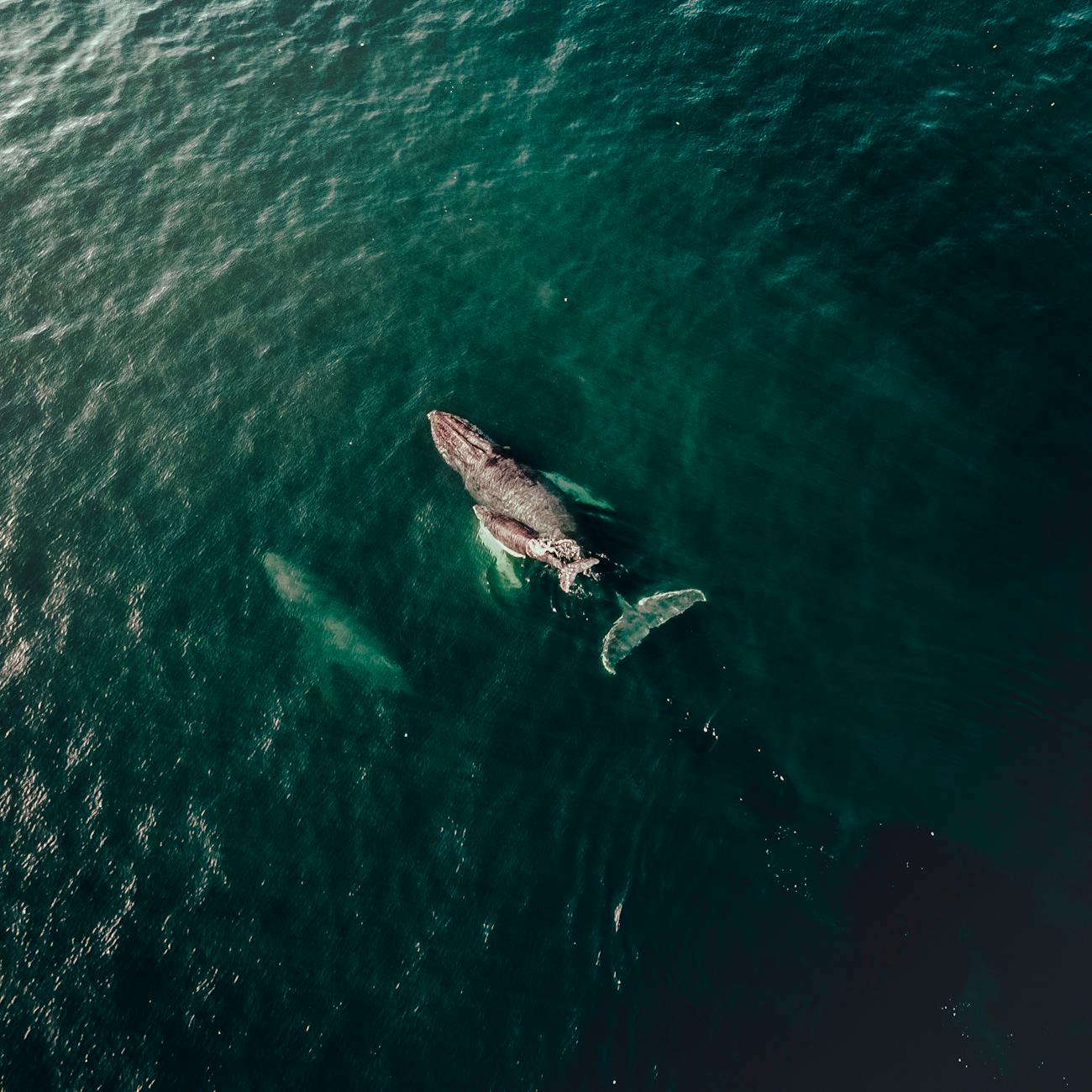
Acoustic frequency refers to the number of pressure oscillations that occur each second in a sound wave and is measured in hertz (Hz). In marine mammal research, frequency determines which species can be detected because different taxa produce vocalizations that occupy distinct frequency bands. For example, the clicks of a sperm whale are concentrated between 1 and 20 kHz, whereas the whistles of a bottlenose dolphin typically range from 5 to 20 kHz. Understanding frequency helps researchers select appropriate recording equipment and design analysis pipelines that capture the relevant spectral content without unnecessary data overload.

Wavelength is the distance between successive points of identical phase in a sound wave, such as crest to crest. It is inversely related to frequency through the equation wavelength = sound speed / frequency. In seawater, where sound travels at roughly 1500 m s⁻¹, a 10 kHz signal has a wavelength of about 0.15 M. Knowledge of wavelength is crucial when configuring hydrophone arrays because the spacing between sensors must be appropriate to avoid spatial aliasing. If hydrophones are placed farther apart than half the wavelength of the target signal, the array may misinterpret the direction of arrival.

Amplitude describes the magnitude of pressure variation in a sound wave and is directly related to perceived loudness. In acoustic measurements, amplitude is often expressed as sound pressure level (SPL) in decibels (dB). Larger amplitude signals are easier to detect against background noise, but they also have the potential to cause disturbance to the animals being studied. Researchers must therefore balance the need for a high signal‑to‑noise ratio (SNR) with ethical considerations regarding acoustic exposure.

Sound pressure level (SPL) quantifies acoustic amplitude on a logarithmic scale using the reference pressure of 1 µPa in water. The formula SPL = 20 log₁₀(p / p₀) yields values in dB re 1 µPa. A typical dolphin whistle may register at 150 dB re 1 µPa, while ambient ocean noise often falls between 90 and 110 dB re 1 µPa. SPL is a foundational metric; it is used to calculate source level, transmission loss, and to assess compliance with marine mammal protection guidelines.

Decibel is the unit that expresses ratios of acoustic quantities on a logarithmic scale. Because the human ear perceives sound intensity logarithmically, decibel notation aligns with perceptual experience and allows a wide range of acoustic energies to be represented compactly. In marine bioacoustics, decibel values are always referenced to the underwater standard of 1 µPa, distinguishing them from air‑based decibel measurements that reference 20 µPa.

Source level is the SPL measured at a standard distance of one meter from the sound source, effectively representing the intrinsic loudness of an animal’s vocalization. Source level is a critical parameter for estimating the detection range of a signal. For instance, a beaked whale click may have a source level of 210 dB re 1 µPa, enabling detection over several kilometers under favorable propagation conditions. Accurate source level estimation requires calibrated equipment and careful correction for transmission loss between the animal and the recorder.

Transmission loss quantifies the reduction in acoustic energy as a sound propagates through the water column. It is expressed in decibels and incorporates spherical spreading (approximately 20 log₁₀(range)) as well as frequency‑dependent absorption. In shallow, sandy environments, additional loss may arise from bottom interaction and scattering. Researchers model transmission loss to predict detection ranges and to design monitoring grids that provide adequate spatial coverage.

Ambient noise encompasses all background acoustic energy unrelated to the target vocalizations. Sources include wind, waves, rain, biological chatter from other species, and anthropogenic activities such as shipping or seismic surveys. Ambient noise levels vary diurnally, seasonally, and with weather conditions. When planning a passive acoustic monitoring (PAM) deployment, investigators must assess typical ambient noise levels to determine the feasibility of detecting low‑amplitude signals.

Signal‑to‑noise ratio (SNR) is the ratio of the target signal’s amplitude to that of the surrounding noise, often expressed in decibels. A high SNR facilitates reliable detection and classification, whereas a low SNR can lead to missed detections or misidentifications. In practice, a SNR of at least 6 dB is commonly required for automated click detectors, while whistle detectors may tolerate slightly lower SNRs due to the longer duration of the signal.

Hydrophone is a transducer that converts underwater pressure fluctuations into electrical voltage. Hydrophones are the primary sensors used in marine mammal bioacoustics. They vary in sensitivity, frequency response, and directional characteristics. A broadband hydrophone capable of recording from 1 Hz to 150 kHz can capture the full repertoire of most cetacean species, while a narrowband hydrophone optimized for low‑frequency baleen whale calls may prioritize sensitivity over a limited range.

Array refers to a spatially distributed set of hydrophones that work together to determine the direction or location of a sound source. Arrays can be linear, planar, or volumetric. The geometry of the array influences its ability to resolve azimuth and elevation angles, as well as its susceptibility to spatial aliasing. For example, a tetrahedral array with hydrophones spaced 0.5 M apart can resolve high‑frequency clicks while maintaining a compact footprint suitable for deployment on a research vessel.

Beamforming is a signal‑processing technique that combines the outputs of multiple hydrophones to enhance signals arriving from a specific direction while suppressing others. This spatial filtering improves SNR and enables precise localization. Real‑time beamforming is often employed on autonomous recorders to reduce data storage requirements by only saving high‑quality detections.

Time difference of arrival (TDOA) measures the relative arrival times of a sound at two or more hydrophones. By solving a set of TDOA equations, the position of the source can be triangulated. Accurate TDOA estimation requires precise clock synchronization among hydrophones, typically achieved with GPS timing or dedicated synchronization cables. Errors in TDOA can arise from clock drift, multipath propagation, or low SNR.

Localization is the process of estimating the three‑dimensional coordinates of a vocalizing animal based on acoustic measurements. Localization methods range from simple two‑hydrophone bearing calculations to sophisticated matched‑field processing that incorporates sound‑speed profiles and bottom topography. The resulting location data can be linked with behavioral observations, environmental variables, or tagging information to explore habitat use.

Click denotes a brief, broadband pulse produced by odontocetes for echolocation and communication. Clicks typically last 10–100 µs and contain energy across a wide frequency range, often extending above 100 kHz in species such as the harbour porpoise. Click analysis involves measuring inter‑click intervals, peak frequency, and source level, which together provide insight into foraging behavior and species identification.

Whistle is a narrowband, frequency‑modulated tonal signal commonly emitted by delphinids during social interactions. Whistles may exhibit complex contour shapes, including upsweeps, downsweeps, and sinusoidal patterns. Spectrogram analysis is the primary tool for visualizing whistles, allowing researchers to extract parameters such as minimum frequency, maximum frequency, and duration for classification.

Pulse refers to a sound that is longer than a click but shorter than a typical song phrase. Many baleen whales produce pulses that are quasi‑periodic and can be used for species identification. Pulse trains from fin whales, for instance, consist of 20‑30 Hz pulses repeated every 10–15 seconds.

Broadband signals contain energy over a wide range of frequencies. Clicks are quintessential broadband sounds, and their analysis often involves computing the full spectrum to capture high‑frequency components. Broadband recordings demand higher sampling rates to avoid aliasing and to preserve fine temporal detail.

Narrowband signals are confined to a limited frequency band, such as whistles or tonal calls. Narrowband recordings can be captured at lower sampling rates, but researchers must ensure that the selected rate still exceeds twice the highest frequency of interest to satisfy the Nyquist criterion.

Spectral analysis encompasses techniques that decompose a sound into its constituent frequencies. The most common method is the fast Fourier transform (FFT), which converts a time‑domain signal into a frequency‑domain representation. Spectral analysis enables measurement of peak frequency, bandwidth, and spectral shape, all of which are diagnostic for species and behavior.

Spectrogram is a visual representation of sound intensity as a function of time and frequency, generated by applying the FFT to successive, overlapping windows of the signal. Spectrograms are indispensable for detecting and classifying vocalizations, particularly tonal calls that exhibit characteristic frequency sweeps. Researchers often annotate spectrograms manually or with automated detection algorithms.

Fast Fourier transform (FFT) is an efficient algorithm that computes the discrete Fourier transform of a signal. By selecting appropriate window length and overlap, the FFT provides a trade‑off between frequency resolution and temporal resolution. For example, a 1024‑sample window at a 250 kHz sampling rate yields a frequency bin width of roughly 244 Hz, suitable for analyzing high‑frequency clicks.

Power spectral density (PSD) describes how power is distributed across frequency bands and is expressed in units of dB re 1 µPa² Hz⁻¹. PSD estimates are useful for characterizing ambient noise, comparing noise environments across sites, and evaluating the impact of anthropogenic sound sources.

Acoustic propagation refers to the physical processes that govern how sound travels through the marine environment. Propagation is affected by sound speed, absorption, scattering, refraction, and boundary interactions. Accurate propagation modeling is essential for predicting detection ranges and for designing mitigation measures for noise impacts.

Refraction occurs when sound waves bend due to spatial variations in sound speed, which in turn are driven by changes in temperature, salinity, and pressure. In the ocean, a typical sound‑speed profile exhibits a minimum at the thermocline, creating a sound channel that can trap low‑frequency energy and enable long‑range transmission. Understanding refraction is vital for interpreting detections that occur far from the source.

Scattering involves the redirection of acoustic energy by particles, bubbles, or rough surfaces. Scattering can increase background noise levels and cause multipath arrivals that complicate localization. In coastal regions with high sediment suspension, scattering may dominate the acoustic environment.

Absorption is the conversion of acoustic energy into heat, primarily due to molecular relaxation processes. Absorption increases with frequency; at 100 kHz, absorption can exceed 1 dB km⁻¹, whereas at 1 kHz it is typically less than 0.01 DB km⁻¹. When planning a survey for high‑frequency clicks, researchers must account for absorption to avoid over‑estimating detection ranges.

Attenuation encompasses all loss mechanisms, including spreading, absorption, and scattering. The term is often used interchangeably with transmission loss but can also refer specifically to the reduction of signal strength due to a particular process.

Oceanographic sound channel is a region of the water column where sound speed gradients create a waveguide that confines acoustic energy. The deep sound channel, located at depths of 800–1200 m in many ocean basins, allows low‑frequency whale calls to travel thousands of kilometers with minimal loss. Knowledge of the sound channel guides the placement of hydrophones for long‑range monitoring.

Bathymetry is the study of underwater depth and topography. Bathymetric features influence acoustic propagation by causing reflections and diffractions. For example, a steep continental slope can produce strong bottom reflections that interfere with direct arrivals, creating a complex interference pattern in the recorded data.

Sound speed profile (SSP) describes how the speed of sound varies with depth. It is derived from measurements of temperature, salinity, and pressure. The SSP is a key input for acoustic propagation models such as ray‑tracing or normal‑mode models. Variations in the SSP over time can lead to changes in detection range, necessitating regular profiling during long‑term monitoring campaigns.

Doppler shift is the change in observed frequency caused by relative motion between the source and the receiver. In marine mammal studies, a moving animal may produce clicks that appear compressed or stretched in time, complicating automated detection. Correcting for Doppler shift improves the accuracy of source‑level estimates and temporal analyses.

Reverberation denotes the persistence of acoustic energy due to multiple reflections from the sea surface, bottom, and other objects. Reverberation can mask weak signals and produce false detections. In shallow water, reverberation is often the dominant source of noise, requiring specialized processing such as matched‑field filtering to isolate target calls.

Masking occurs when background noise or other sounds obscure a target signal, reducing its effective SNR. Masking thresholds are species‑specific; some cetaceans can detect signals that are only a few decibels above ambient noise, while others require larger margins. Understanding masking informs the design of detection algorithms and the interpretation of absence data.

Passive acoustic monitoring (PAM) is the practice of listening to the marine environment without emitting sound, relying solely on hydrophones to record vocalizations and ambient noise. PAM is widely used for long‑term, non‑invasive surveys of cetacean presence, distribution, and seasonal patterns. Deployments may be fixed (e.G., Moored buoys) or mobile (e.G., Towed arrays).

Active acoustic surveying involves transmitting sound pulses and listening for echoes, typically for fisheries assessment or seafloor mapping. While active methods can provide complementary data on prey distribution, they must be carefully managed to avoid disturbing marine mammals. Researchers often coordinate active surveys with PAM to monitor potential impacts in real time.

Tag in this context refers to a biologging device that records acoustic, movement, and environmental data from an individual animal. Acoustic tags may include a hydrophone positioned near the animal’s head, allowing researchers to capture on‑body vocalizations and the acoustic scene as perceived by the animal. Tag data can be synchronized with ambient recordings to study sound exposure.

Data logger is a device that stores sensor measurements over time. In marine bioacoustics, data loggers are embedded in tags, autonomous recorders, or moorings. They often feature solid‑state memory and programmable sampling schedules to optimize battery life while capturing periods of interest.

Sampling rate defines how many times per second a continuous acoustic signal is digitized. According to the Nyquist theorem, the sampling rate must be at least twice the highest frequency of interest to avoid aliasing. For recordings intended to capture 150 kHz clicks, a minimum sampling rate of 300 kHz is required, though many researchers opt for 500 kHz to provide a safety margin.

Nyquist frequency is half the sampling rate and represents the highest frequency that can be accurately represented without aliasing. When the Nyquist frequency is exceeded, higher‑frequency components fold back into lower frequencies, creating erroneous spectral artifacts that can masquerade as biological signals.

Aliasing is the distortion that occurs when a signal contains frequency components above the Nyquist limit. In practice, aliasing can generate spurious peaks in a spectrogram that may be misidentified as clicks or whistles. Anti‑aliasing filters (low‑pass) are therefore applied before digitization to suppress frequencies beyond the Nyquist limit.

Quantization is the process of mapping a continuous voltage amplitude to a discrete set of digital values, determined by the bit depth of the analog‑to‑digital converter (ADC). Higher bit depth provides greater dynamic range and reduces quantization noise. A 16‑bit ADC yields a theoretical dynamic range of about 96 dB, sufficient for most marine mammal recordings, though 24‑bit systems are increasingly used for high‑fidelity research.

Dynamic range is the ratio between the largest and smallest detectable acoustic pressures, expressed in decibels. It is limited by the ADC bit depth, preamplifier gain, and system noise floor. Ensuring an adequate dynamic range prevents both clipping of loud clicks and loss of faint calls in noisy environments.

Calibration is the procedure of determining the exact relationship between recorded voltage and actual sound pressure. Calibration involves exposing the hydrophone to a known acoustic source, such as a pistonphone, and measuring the system’s response. Regular calibration is essential for comparing SPL values across studies and for meeting regulatory standards.

Gain refers to the amplification applied to the hydrophone signal before digitization. Adjustable gain allows researchers to optimize the signal level for a given acoustic environment. However, excessive gain can introduce distortion, while insufficient gain reduces SNR. Careful gain setting, often guided by pre‑deployment tests, balances these trade‑offs.

Preamplifier is an electronic component that boosts the weak voltage output of a hydrophone to a level suitable for the ADC. Low‑noise preamplifiers are preferred because they add minimal additional noise, preserving the SNR of the original signal. In some autonomous recorders, the preamplifier is integrated into the hydrophone housing.

Filter is a signal‑processing tool that attenuates specific frequency ranges while allowing others to pass. Common filter types include high‑pass, low‑pass, band‑pass, and notch filters. Filters are applied to remove unwanted noise (e.G., Low‑frequency ship noise) or to isolate a frequency band of interest (e.G., The 20 kHz peak of a dolphin whistle).

High‑pass filter removes frequencies below a designated cutoff, often employed to eliminate low‑frequency ocean noise and improve detection of higher‑frequency clicks. A typical high‑pass setting for dolphin studies might be 5 kHz.

Low‑pass filter suppresses frequencies above a cutoff, useful when focusing on low‑frequency baleen whale calls. For example, a low‑pass filter with a cutoff at 200 Hz can isolate fin whale moans while discarding higher‑frequency noise.

Band‑pass filter combines high‑ and low‑pass characteristics to retain a specific frequency band. Researchers might apply a band‑pass filter from 8 to 30 kHz to isolate harbour porpoise clicks while rejecting both low‑frequency noise and ultrasonic interference.

Notch filter targets a narrow frequency band for attenuation, often used to remove power‑line interference at 60 Hz or to suppress tonal noise from a nearby vessel’s propeller. Notch filters must be applied judiciously to avoid inadvertently removing biologically relevant frequencies.

Windowing involves multiplying a segment of the time‑domain signal by a weighting function (window) before performing an FFT. Windowing reduces spectral leakage, which is the spreading of energy from a strong frequency component into adjacent bins. Common windows include Hamming, Hann, and Blackman. Selecting an appropriate window balances leakage reduction against frequency resolution loss.

Leakage occurs when the finite length of a data segment causes discontinuities at its edges, leading to smearing of spectral energy. Leakage can obscure weak signals and create false peaks. Proper windowing and sufficient segment length mitigate this effect.

Spectral resolution is the ability to distinguish closely spaced frequency components and is determined by the length of the FFT window. Longer windows provide finer resolution but reduce temporal resolution. Researchers often experiment with different window lengths to optimize detection of specific vocalization types.

Temporal resolution describes how precisely the timing of events can be resolved in a recording. High temporal resolution is essential for measuring inter‑click intervals and for aligning acoustic data with behavioral observations. Short window lengths and high sampling rates improve temporal resolution at the cost of spectral detail.

Duty cycle is the proportion of time that a recorder is actively sampling versus idle. Duty‑cycled recordings, such as 5 minutes on / 55 minutes off, extend battery life and storage capacity, allowing longer deployments. However, duty cycling may miss brief vocalizations, introducing bias in occurrence estimates.

Recording schedule defines the timing and duration of data acquisition. Researchers design schedules based on target species’ vocal activity patterns, battery constraints, and data storage limits. For example, a schedule that records during dusk and dawn aligns with the crepuscular peak in humpback whale song activity.

Deployment refers to the act of placing a hydrophone system in the marine environment. Deployments can be fixed (e.G., Anchored to the seafloor), mobile (e.G., Towed behind a vessel), or autonomous (e.G., Attached to a buoy). Each deployment type presents distinct logistical challenges, such as securing cables in strong currents or ensuring GPS connectivity for surface buoys.

Mooring is a structure used to anchor a hydrophone or recorder to the seabed while allowing vertical movement with tides and currents. Moorings often include a buoyant float, a weight, and a cable with a hydrophone attached at a predetermined depth. Proper mooring design minimizes self‑noise caused by cable vibration and motion.

Buoy can serve as a surface platform for hydrophones, power supplies, and telemetry equipment. Buoys are equipped with solar panels or batteries to extend deployment duration. Surface buoys also provide a convenient location for retrieving data via wireless links, reducing the need for diver retrieval.

Autonomous recorder is a self‑contained system that captures acoustic data without real‑time human oversight. These devices typically incorporate a hydrophone, preamplifier, ADC, storage, and power source. Autonomous recorders are essential for long‑term monitoring in remote or deep‑water locations.

Data management encompasses the processes of organizing, storing, backing up, and sharing acoustic datasets. Effective data management includes establishing consistent file naming conventions, maintaining metadata records, and employing version control for analysis scripts. Proper data stewardship facilitates reproducibility and enables collaboration across institutions.

Metadata provides contextual information about each recording, such as deployment location, depth, date, time, sampling parameters, and calibration details. Metadata is critical for interpreting acoustic measurements and for integrating datasets from multiple projects. Standards such as the International Association for the Physical Sciences of the Ocean (IAPSO) guidelines help ensure metadata completeness.

Archiving involves preserving raw and processed acoustic data for long‑term accessibility. Archiving may be performed in institutional repositories, national data centers, or cloud storage platforms. Researchers must consider data formats (e.G., WAV, FLAC) and documentation to guarantee future usability.

Annotation is the process of marking timestamps and labeling acoustic events within recordings. Annotations may indicate the presence of clicks, whistles, or anthropogenic noises, and can include confidence scores. Manual annotation provides high accuracy but is time‑consuming; thus, many projects employ semi‑automated tools to assist annotators.

Automated detection uses algorithms to identify vocalizations without human intervention. Detection methods range from simple energy‑threshold approaches to sophisticated machine‑learning classifiers. Automated detection accelerates data processing, enabling researchers to handle the massive volumes generated by continuous PAM deployments.

Machine learning encompasses computational techniques that allow algorithms to learn patterns from data. In bioacoustics, supervised learning models are trained on labeled examples of clicks or whistles to recognize similar patterns in new recordings. Unsupervised methods can cluster unknown sounds, potentially revealing previously undocumented vocalization types.

Convolutional neural network (CNN) is a deep‑learning architecture particularly effective for image‑like data such as spectrograms. CNNs automatically extract hierarchical features, making them well suited for classifying complex whale songs or distinguishing overlapping vocalizations. Training a CNN requires a large, curated dataset and substantial computational resources.

Feature extraction is the step of converting raw acoustic data into a set of descriptive variables (features) that capture relevant characteristics. Common features include peak frequency, bandwidth, duration, modulation rate, and spectral centroid. Feature extraction reduces data dimensionality, facilitating classification and statistical analysis.

Classification assigns each detected acoustic event to a predefined category, such as species or call type. Classification can be performed using rule‑based decision trees, support vector machines, or deep‑learning models. Accuracy depends on the quality of training data, the relevance of features, and the diversity of acoustic contexts.

False positive occurs when a detection algorithm incorrectly identifies noise as a target signal. High false‑positive rates increase the workload for manual verification and may inflate estimates of animal presence. Strategies to reduce false positives include raising detection thresholds, incorporating multi‑feature criteria, and applying post‑processing filters.

False negative is the failure to detect a genuine vocalization. False negatives lead to underestimation of occurrence and can bias ecological inferences. Mitigation measures involve lowering detection thresholds, improving SNR through beamforming, and ensuring adequate coverage of the acoustic environment.

Validation assesses the performance of detection and classification algorithms by comparing automated results with a ground‑truth dataset, typically generated through manual annotation. Metrics such as precision, recall, and F‑score quantify accuracy. Validation is an iterative process; insights gained from errors guide algorithm refinement.

Inter‑observer reliability measures the consistency between different human annotators. High reliability indicates that the annotation protocol is clear and that the vocalizations are distinct enough to be identified by multiple observers. Calculating Cohen’s kappa or Fleiss’ kappa provides statistical evidence of agreement.

Acoustic indices are quantitative metrics that summarize properties of the soundscape, such as acoustic diversity, entropy, or biophony‑to‑anthropophony ratios. Indices can be used to monitor ecosystem health, detect changes over time, and assess the impact of human activities. While useful for broad assessments, indices lack the specificity of species‑level identification.

Biodiversity metrics derived from acoustic data may include species richness estimates based on detection events, vocal activity patterns, and temporal overlap of calls. Acoustic methods can complement visual surveys, especially in low‑visibility conditions or for cryptic species.

Acoustic footprint describes the spatial extent of sound generated by a source, such as a vessel or seismic air gun, and its potential to affect marine mammals. Mapping acoustic footprints involves modeling propagation, accounting for source level, frequency content, and environmental conditions. Footprint analyses inform mitigation strategies like exclusion zones.

Soundscape encompasses the entire acoustic environment, integrating natural biophony, geophony, and anthropogenic noise. Researchers analyze soundscapes to understand how background noise influences animal communication, behavior, and habitat selection. Seasonal and diel variations in the soundscape can be visualized using spectrogram mosaics.

Anthropogenic noise originates from human activities and includes shipping, construction, sonar, and seismic surveys. These sounds can cause masking, behavioral changes, and physiological stress in marine mammals. Quantifying anthropogenic noise levels is a prerequisite for impact assessments and for developing mitigation measures.

Shipping noise is dominated by low‑frequency (10–300 Hz) broadband energy generated by propeller cavitation and engine vibrations. Shipping lanes often create persistent noise corridors that overlap with the frequency bands of baleen whale calls, leading to chronic masking. Researchers may use AIS (Automatic Identification System) data to correlate ship traffic with acoustic measurements.

Sonar systems emit focused acoustic beams for navigation, fish detection, or military purposes. Sonar pulses can be high‑intensity and cover frequencies overlapping with cetacean communication bands, raising concerns about disturbance. Controlled exposure experiments (CEEs) are sometimes conducted to evaluate behavioral responses to sonar.

Seismic surveys employ air‑gun arrays that release high‑energy bubbles, producing low‑frequency (10–200 Hz) sound that propagates over long distances. Seismic operations have been linked to altered migration routes and temporary displacement of whales. Regulatory agencies often require mitigation measures such as shutdown zones and ramp‑up procedures.

Mitigation refers to actions taken to reduce the adverse effects of anthropogenic sound on marine mammals. Common mitigation strategies include establishing exclusion zones, adjusting source level or timing, using bubble curtains, and implementing real‑time acoustic monitoring to trigger shutdowns when animals approach. Effective mitigation relies on accurate detection and rapid response capabilities.

Impact assessment evaluates the potential consequences of a noise source on marine mammals, integrating acoustic exposure models, behavioral data, and population-level effects. Impact assessments are required for permitting processes and inform management decisions. They may employ dose‑response relationships derived from previous studies to predict behavioral changes.

Tagging in the context of bioacoustics often involves attaching a suction‑cup or dart‑mounted acoustic tag to a free‑ranging animal. Tags capture on‑body sound, movement, and environmental parameters such as temperature and depth. Tag data provide unique insight into the soundscape experienced by the animal and can reveal fine‑scale foraging behavior not observable from remote sensors.

Tag deployment requires careful consideration of animal welfare, attachment duration, and data retrieval methods. Researchers must balance the desire for high‑resolution data with the need to minimize stress and tag loss. Tag retrieval can be facilitated by acoustic release mechanisms that allow the tag to detach and float to the surface.

Acoustic footprint mapping combines source level measurements, propagation modeling, and bathymetric data to produce spatial representations of sound exposure levels. These maps are used by regulators to define zones where sound exceeds thresholds for marine mammal hearing groups. They also help researchers assess cumulative exposure from multiple sources.

Calibration standards such as the International Standards Organization (ISO) pistonphone provide reference pressures for verifying hydrophone response. Regular calibration before and after field deployments ensures data comparability and helps identify sensor drift or damage.

Signal processing pipeline typically begins with raw voltage data, followed by filtering, gain correction, and conversion to SPL. Subsequent steps include segmentation, feature extraction, detection, and classification. Each stage introduces potential sources of error; therefore, documentation of processing parameters is essential for reproducibility.

Pre‑processing may involve removing DC offsets, applying anti‑aliasing filters, and correcting for sensor tilt. In coastal environments, wave‑induced motion can introduce low‑frequency noise that is mitigated by high‑pass filtering. Pre‑processing also includes synchronizing multiple channels when working with arrays.

Matched‑field processing utilizes detailed environmental models to predict the acoustic field at each hydrophone for a given source location. By comparing measured data with model predictions, matched‑field techniques can achieve high‑precision localization even in complex environments. However, they require accurate SSPs and bottom properties, which may be difficult to obtain in dynamic coastal settings.

Real‑time monitoring systems stream acoustic data to shore stations for immediate analysis. Real‑time detection enables rapid response to the presence of protected species during noisy activities, such as naval exercises. Implementing real‑time monitoring demands reliable telemetry, low‑latency processing algorithms, and robust power supplies.

Data compression reduces storage requirements by encoding audio with fewer bits while preserving essential information. Lossless formats like FLAC retain the full acoustic fidelity needed for scientific analysis, whereas lossy formats (e.G., MP3) may discard subtle spectral details critical for species identification. Researchers must weigh storage constraints against the need for high‑quality data.

Statistical analysis of acoustic datasets may involve occupancy modeling, generalized linear models, or time‑series analysis to relate vocal activity to environmental covariates. Advanced techniques such as hierarchical Bayesian models can incorporate uncertainty in detection probability and account for spatial autocorrelation.

Occupancy modeling estimates the probability that a species is present at a site, correcting for imperfect detection. In acoustic surveys, detection probability is a function of SNR, source level, and environmental conditions. Incorporating detection probability yields more reliable estimates of distribution and abundance.

Temporal autocorrelation arises when consecutive acoustic samples are not independent, such as when a whale produces a series of clicks. Ignoring autocorrelation can inflate type‑I error rates in statistical tests. Researchers address this by subsampling data, using block bootstrapping, or incorporating autocorrelation structures into models.

Cross‑validation assesses the generalizability of a classification model by partitioning data into training and testing subsets. K‑fold cross‑validation, where the dataset is divided into K equal parts, provides a robust estimate of model performance while making efficient use of limited labeled data.

Transfer learning leverages models trained on one dataset to improve performance on another, reducing the need for extensive labeled data. In marine bioacoustics, a CNN trained on a large dataset of dolphin whistles can be fine‑tuned to detect similar signals in a new geographic region, accelerating the development of detection tools.

Ethical considerations include minimizing acoustic disturbance, ensuring animal welfare during tagging, and respecting data ownership and indigenous knowledge. Researchers must obtain appropriate permits, follow best practices for acoustic exposure, and engage with local stakeholders when planning deployments.

Regulatory frameworks such as the U.S. Marine Mammal Protection Act (MMPA) and the International Maritime Organization (IMO) guidelines dictate permissible sound levels and required mitigation measures. Compliance involves documenting exposure metrics, conducting impact assessments, and maintaining records of mitigation actions.

Challenges in tropical waters include high ambient noise from wind‑driven surface waves, complex bathymetry, and rapid changes in the sound‑speed profile due to temperature gradients. These factors increase propagation variability and complicate detection. Adaptive deployment strategies, such as seasonal timing and depth selection, help mitigate these challenges.

Challenges in deep‑sea environments involve limited power for long deployments, the need for pressure‑resistant housings, and difficulties in retrieving equipment. Low temperatures can affect battery performance, and the absence of surface access necessitates autonomous operation for months. Emerging technologies like energy‑harvesting buoys aim to address these constraints.

Data volume management is a practical concern; high‑sampling‑rate recordings generate terabytes of data per deployment. Efficient data handling includes on‑board processing to discard irrelevant segments, hierarchical storage systems, and cloud‑based analysis pipelines. Metadata tagging enables rapid retrieval of specific events.

Interdisciplinary collaboration enhances bioacoustic research by integrating oceanography, engineering, ecology, and computer science.