Fundamentals Of CFD Markets

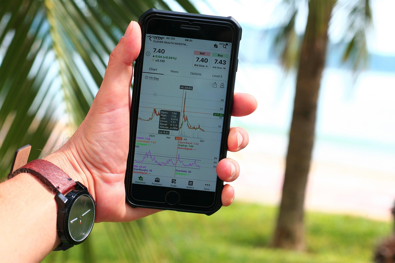
CFD stands for contract for difference. It is a derivative that allows traders to speculate on the price movement of an underlying asset without owning the asset itself. For example, if a trader believes the price of gold will rise, they can buy a gold CFD. If the price increases, the trader receives the difference between the opening and closing prices; if it decreases, the trader pays that difference. The key advantage is the ability to go long or short with the same instrument, which makes CFDs especially suitable for algorithmic strategies that seek to capture both upward and downward trends.

Underlying asset refers to the real‑world security or commodity that the CFD mirrors. Common underlying assets include equities, indices, commodities, foreign exchange pairs, and cryptocurrencies. When designing an algorithm, the choice of underlying asset determines the data requirements, market hours, and volatility characteristics. For instance, a CFD on the S&P 500 index will be affected by the U.S. Market calendar, whereas a CFD on EUR/USD will follow the forex trading day, which is essentially 24‑hour.

Spread is the difference between the bid price (what a trader can sell for) and the ask price (what a trader can buy for). In CFD markets, the spread is a primary source of cost. A typical EUR/USD CFD spread might be 0.2 Pips, while a more exotic pair could have a spread of 1.5 Pips. Algorithms that trade very frequently, such as scalping bots, must incorporate spread cost into their profitability calculations, otherwise the strategy may appear profitable on paper but lose money in execution.

Pip stands for “percentage in point” and represents the smallest price increment for most forex‑related CFDs. In most currency pairs, one pip equals 0.0001 Of the quoted price. For example, if EUR/USD moves from 1.1200 To 1.1201, The change is one pip. When coding a strategy, it is common to express profit targets and stop‑loss levels in pips because they provide a standardized measure across different instruments.

Lot size defines the quantity of the underlying asset represented by a single CFD contract. In forex, a standard lot is 100,000 units of the base currency, a mini‑lot is 10,000, and a micro‑lot is 1,000. If a trader opens a CFD for 2 mini‑lots of EUR/USD, the notional exposure is 20,000 euros. Algorithms that dynamically adjust position size based on volatility often use the lot size concept to calculate the appropriate number of contracts for each trade.

Margin is the amount of capital a trader must deposit to open a CFD position. Because CFDs are leveraged, the margin required is only a fraction of the total notional exposure. For example, a 5 % margin requirement on a $100,000 position means the trader needs to post $5,000. In algorithmic trading, margin is a critical constraint; the system must monitor available margin in real time to avoid exceeding the broker’s limits.

Leverage amplifies both potential gains and potential losses. A leverage of 20:1 Means that for every $1 of margin, the trader controls $20 of notional exposure. If a CFD on a stock moves 2 % in the trader’s favor, the profit on the margin is 40 % (2 % × 20). Conversely, a 2 % adverse move wipes out the entire margin. Algorithms that use high leverage must incorporate strict risk controls, such as maximum drawdown limits, to prevent catastrophic loss.

Margin call occurs when the equity in a trading account falls below the required maintenance margin. The broker demands additional funds to keep positions open. In an automated system, a margin‑call detection routine should trigger immediate position reduction or closure to protect the account. Failure to handle margin calls programmatically can result in forced liquidation at unfavorable prices.

Stop loss is an order placed to exit a position if the market moves against the trader beyond a predefined level. For example, a trader who buys a CFD on Apple at $150 might set a stop loss at $145 to limit loss to $5 per share. In algorithmic implementations, stop‑loss levels are often expressed in pips, percentages, or volatility‑adjusted measures such as the average true range (ATR). Proper placement of stop losses is essential for controlling downside risk.

Take profit (or profit target) is the opposite of a stop loss: An order that closes a position once a predefined profit level is reached. Continuing the Apple example, a take‑profit order might be set at $160, securing a $10 gain per share. Automated strategies frequently use a risk‑to‑reward ratio, such as 1:2, Meaning the take‑profit distance is twice the stop‑loss distance, to ensure statistically positive expectancy.

Long position means buying a CFD with the expectation that the underlying price will rise. The trader profits when the market moves up. Conversely, a short position involves selling a CFD first, anticipating a price decline; profit is realized if the market falls. Algorithmic strategies can be designed to be market‑neutral by simultaneously holding long and short positions in correlated assets, thereby reducing exposure to overall market direction.

Market order instructs the broker to execute a trade immediately at the best available price. It guarantees execution but not price, which can be problematic in fast‑moving markets where slippage may occur. An algorithm that relies on precise entry levels may prefer limit orders instead.

Limit order specifies a maximum price for buying or a minimum price for selling. The order will only fill if the market reaches the specified price. For instance, a trader may place a buy limit order at 1.1150 For EUR/USD, ensuring they only enter if the price falls to that level. Limit orders help control entry price but carry the risk of non‑execution if the market never reaches the level.

Stop order (sometimes called a stop‑limit) becomes a market order once a trigger price is breached. A sell stop placed above the current price can be used to protect a short position, while a buy stop above the current price can be used to enter a long position on a breakout. In algorithmic code, stop orders are often used to automate breakout strategies.

Slippage is the difference between the expected execution price and the actual filled price. It commonly occurs during high volatility or low liquidity. For example, a trader expecting to buy EUR/USD at 1.1200 May actually receive 1.1203, Incurring a 3‑pip slippage. Algorithms must model slippage, perhaps by adding a fixed or variable buffer to the expected price, to produce realistic performance estimates.

Liquidity measures how easily an asset can be bought or sold without causing a significant price change. Highly liquid CFDs, such as those on major indices, typically have narrow spreads and low slippage. Illiquid CFDs, like those on exotic commodities, may exhibit wide spreads and large price gaps. Liquidity considerations affect order sizing, execution venue selection, and risk management.

Volatility quantifies the rate at which the price of an underlying asset changes. It is often measured by the standard deviation of returns or by the average true range (ATR). High volatility offers larger profit opportunities but also higher risk. Algorithms may adapt position size based on recent volatility, a technique known as volatility scaling, to maintain a consistent risk profile.

Bid‑ask spread is synonymous with “spread” but emphasizes the two components: The bid price (what the broker will buy from the trader) and the ask price (what the broker will sell to the trader). In CFD markets, the spread can widen during news releases, leading to higher transaction costs. A robust algorithm monitors spread changes and may pause trading during periods of abnormal widening.

Overnight financing (also called rollover or swap) is the cost or credit applied to positions held open beyond the market’s daily settlement time. For a CFD, the broker typically charges interest based on the underlying asset’s financing rate and the notional amount. For example, a long position on a gold CFD might incur a daily financing charge of 0.01 % Of the notional value. Algorithms that hold positions for multiple days must factor financing costs into the profitability model.

Rollover refers to the process of extending a contract’s expiry by paying or receiving the overnight financing. In CFD platforms that offer “daily rollover,” the position automatically continues, and the financing is applied each night. Traders who use swing‑trading or trend‑following strategies need to account for cumulative financing charges, especially when the strategy involves high leverage.

Funding rate is the percentage used to calculate overnight financing. It can be positive (cost) or negative (credit) depending on the direction of the position and the underlying asset’s interest rate differentials. For example, a CFD on a currency pair where the base currency has a higher interest rate than the quote currency will often provide a credit to long positions. Understanding funding rates helps in selecting assets where the financing cost aligns with the expected holding period.

Execution speed measures how quickly an order reaches the market and is filled. In high‑frequency algorithmic trading, execution latency measured in microseconds can be decisive. Even a few milliseconds of delay can cause missed opportunities or adverse price movement. Traders may choose low‑latency brokers, colocated servers, or direct market access (DMA) to reduce execution time.

Algorithmic strategy is a systematic set of rules that dictate entry, exit, risk management, and position sizing. Common categories include mean‑reversion, trend‑following, breakout, statistical arbitrage, and market‑making. Each strategy type has distinct data requirements and performance expectations. For instance, a mean‑reversion strategy might rely on short‑term price oscillations, while a trend‑following strategy looks for sustained directional moves.

Mean reversion assumes that prices tend to return to an average value over time. A typical implementation uses the moving average as a reference: When price deviates significantly above the average, the algorithm shorts; when it falls below, the algorithm goes long. The effectiveness of mean‑reversion depends on the asset’s tendency to oscillate rather than trend, and on the chosen look‑back period. Over‑fitting the averaging window can lead to poor out‑of‑sample performance.

Trend following exploits the tendency of markets to move in persistent directions. Strategies often employ moving‑average crossovers, breakout detection, or momentum indicators such as the Relative Strength Index (RSI). For example, a simple trend‑following system might buy when the 20‑day moving average crosses above the 50‑day moving average and sell when the opposite occurs. Trend‑following strategies are generally more robust in trending markets but can suffer during sideways periods.

Arbitrage seeks to profit from price discrepancies between two or more markets. In CFD contexts, triangular arbitrage can arise when the implied cross‑rate derived from two CFDs differs from the directly quoted CFD. For example, if CFD A represents EUR/USD, CFD B represents USD/JPY, and CFD C represents EUR/JPY, an arbitrageur can trade the three to lock in a risk‑free profit if the relationship deviates from the theoretical one. Implementing arbitrage requires ultra‑low latency and precise synchronization of data feeds.

Market making involves providing liquidity by continuously posting bid and ask quotes. Market‑making algorithms earn the spread while managing inventory risk. In CFD markets, some brokers act as market makers, but independent traders can also adopt a market‑making approach by placing limit orders on both sides of the order book. The key challenges include inventory control, adverse selection, and exposure to large price moves.

Order book displays the list of all outstanding limit orders at various price levels. Depth of market (DOM) data shows the quantity available at each price. Algorithms that analyze the order book can infer short‑term supply‑demand imbalances. For instance, a sudden surge of buy orders at a price level might indicate an imminent upward move, prompting a short‑term long entry.

Depth of market (DOM) is a detailed view of the order book, typically showing the top five or ten price levels on each side. Traders use DOM to gauge market pressure and to place iceberg orders that hide true order size. In CFD platforms that expose DOM, algorithmic traders can implement “order‑flow” strategies that react to real‑time changes in liquidity.

Tick size is the smallest price increment allowed for a CFD. For most forex CFDs, the tick size is one pip (0.0001), But some platforms allow fractional pips (e.G., 0.5 Pip). Tick size influences the granularity of stop‑loss and take‑profit placement. When coding an algorithm, it is essential to round price levels to the nearest permissible tick to avoid order rejections.

Tick value translates a one‑tick movement into monetary terms. In a CFD on a 100‑lot of EUR/USD, one pip (one tick) equals $10. Knowing tick value allows the algorithm to calculate profit and loss in currency terms and to size positions appropriately relative to risk limits.

Risk management encompasses all techniques used to protect capital. Core components include position sizing, stop‑loss placement, diversification, and drawdown control. A common rule is to risk no more than 1 % of account equity on any single trade. An algorithm can enforce this rule by dynamically adjusting lot size based on the distance to the stop loss and the desired risk amount.

Position sizing determines how many contracts to trade for each signal. Methods range from fixed lot size to volatility‑adjusted sizing. For example, a volatility‑scaled approach might calculate the position size as (Risk % × Equity) / (ATR × Contract Multiplier). This ensures that each trade contributes a similar amount of risk to the portfolio, regardless of the underlying’s price level.

Exposure is the total notional value of open positions. High exposure can amplify gains but also magnify losses and increase margin requirements. Algorithms often limit exposure to a percentage of total equity, especially when trading multiple instruments simultaneously, to prevent concentration risk.

Drawdown measures the decline from a portfolio’s peak equity to its lowest point before a new peak is reached. It is expressed as a percentage. A strategy with a 20 % maximum drawdown may be unsuitable for risk‑averse investors. Automated systems can incorporate drawdown monitoring, automatically halting trading if drawdown exceeds a predefined threshold.

Equity curve plots the cumulative profit and loss of a strategy over time. It visualizes periods of growth, stagnation, and drawdown. Traders use the equity curve to assess consistency and to detect regime changes. A smooth, upward‑sloping equity curve with low volatility is generally preferable to one with sharp spikes.

Backtesting evaluates a strategy’s performance using historical data. It involves simulating trades as if the algorithm had run in the past, applying the same entry, exit, and risk rules. Critical considerations include data quality, handling of slippage, and realistic modeling of transaction costs. A well‑executed backtest provides confidence but does not guarantee future success.

Forward testing (or paper trading) applies the algorithm to live market data without committing real capital. It validates whether the strategy behaves as expected in a live environment, accounting for real‑time data latency and order execution nuances. Forward testing bridges the gap between backtesting and live deployment.

Overfitting occurs when a model captures noise rather than the underlying signal. An overfitted algorithm may achieve spectacular backtest results but fail miserably in live trading. Techniques to avoid overfitting include using out‑of‑sample data, limiting the number of parameters, and applying regularization methods.

Data snooping refers to the practice of mining historical data until a desirable result is found, then treating that result as a robust pattern. It inflates the perceived performance of a strategy. To mitigate data snooping, traders should pre‑define hypotheses, use proper statistical tests, and maintain a disciplined research workflow.

Latency is the delay between the moment a market event occurs and the moment the algorithm receives or reacts to it. Sources of latency include data feed transmission, processing time, and order routing. In high‑frequency CFD trading, even microsecond latency differences can be decisive. Reducing latency may involve colocating servers near the broker’s data center or using ultra‑low‑latency APIs.

High‑frequency trading (HFT) describes strategies that execute a large number of trades within very short timeframes, often milliseconds or microseconds. HFT in CFD markets typically focuses on exploiting minute price inefficiencies, order‑book imbalances, or latency arbitrage. Implementing HFT requires specialized infrastructure, such as FPGA‑based order execution and direct market access.

Order flow analysis examines the stream of incoming orders to infer market direction. A surge of aggressive buy orders may indicate buying pressure, prompting a short‑term long entry. Algorithms that ingest order‑flow data need to process high‑volume messages efficiently and filter out noise, often employing statistical smoothing techniques.

Transaction cost analysis (TCA) quantifies the total cost of trading, including spreads, commissions, slippage, and market impact. A strategy that appears profitable before costs can become unprofitable after TCA. Incorporating TCA into backtesting ensures that performance metrics reflect realistic net returns.

Partial fill occurs when only a portion of an order is executed, typically due to insufficient liquidity at the requested price. Algorithms must handle partial fills gracefully, either by adjusting remaining order parameters or by aggregating multiple fills to complete the intended position size.

Order queue represents the sequence of pending orders at a given price level. When many orders sit in the queue, execution may be delayed, especially for large market orders. Understanding the order queue helps in estimating execution latency and potential price impact.

Market impact is the price movement caused by a trader’s own order. Large orders can move the market against the trader, eroding expected profits. Algorithms can reduce market impact by splitting large orders into smaller slices (order slicing) and spreading them over time, a technique known as “iceberg” ordering.

Hedging involves opening offsetting positions to reduce risk. In CFD markets, a trader might hedge a long equity CFD with a short index CFD that is positively correlated, thereby mitigating exposure to market‑wide moves. Hedging can also be used to protect against currency risk when trading non‑domestic assets.

Correlation measures how two assets move relative to each other, typically expressed by the Pearson correlation coefficient. A correlation of +0.9 Indicates strong co‑movement, while –0.9 Indicates strong inverse movement. Algorithms that trade multiple CFDs often diversify by selecting assets with low or negative correlations to reduce portfolio volatility.

Diversification spreads capital across different instruments, sectors, or strategies to lower overall risk. In CFD portfolios, diversification may involve combining equity CFDs, commodity CFDs, and forex CFDs. While diversification reduces unsystematic risk, it does not eliminate systematic market risk.

Regulatory environment governs how CFD trading is conducted, including leverage caps, client protection rules, and reporting obligations. For example, the European Securities and Markets Authority (ESMA) limits retail CFD leverage to 30:1 On major indices. Algorithms must be designed to respect jurisdiction‑specific restrictions, such as prohibiting certain order types or limiting exposure.

Compliance ensures that trading activities adhere to legal and internal policies. Automated systems should incorporate checks for prohibited instruments, maximum leverage, and anti‑money‑laundering (AML) thresholds. Non‑compliance can result in fines, account suspension, or legal action.

KYC (Know Your Customer) procedures verify the identity of clients and assess risk. While KYC is primarily a broker responsibility, algorithmic traders who manage client funds must ensure that all accounts have completed KYC to avoid regulatory breaches.

AML (Anti‑Money Laundering) regulations require monitoring for suspicious transaction patterns. Automated trading platforms often embed AML filters that flag large or unusual CFD trades for review. Developers should design logging mechanisms that capture sufficient detail for AML audits.

Trade execution venue is the location or network through which orders are routed. Options include electronic communication networks (ECNs), straight‑through processing (STP) brokers, and market‑making platforms. The choice of venue affects latency, spread, and the likelihood of order fill. Algorithms may route orders dynamically based on venue performance metrics.

ECN (Electronic Communication Network) aggregates liquidity from multiple participants, offering transparent pricing and typically tighter spreads. ECN brokers often charge a commission per trade, which must be accounted for in profitability calculations.

STP (Straight‑Through Processing) routes orders directly to liquidity providers without manual intervention. STP brokers may offer variable spreads that widen during volatile periods. Understanding the broker’s execution model helps in anticipating spread behavior.

Broker acts as the intermediary that provides CFD access, margin financing, and order execution. Broker selection criteria include regulation, reliability, spread competitiveness, API quality, and available leverage. An algorithmic trader should test multiple brokers in a sandbox environment before committing capital.

Synthetic instrument describes a CFD that replicates the payoff of a complex underlying, such as a basket of stocks or a custom index. Synthetic CFDs enable exposure to diversified assets without needing to trade each component individually. Programming a strategy for a synthetic CFD may require handling the basket’s constituent weighting and rebalancing schedule.

Price feed delivers real‑time market data to the algorithm. High‑quality price feeds provide low latency, accurate bid/ask quotes, and depth‑of‑market information. Data feed reliability is essential; a feed outage can cause missed trades or unintended positions. Redundant feeds and heartbeat monitoring improve resilience.

Historical data is used for backtesting and model training. It must be clean, with correct timestamps, corporate actions (e.G., Dividends, splits), and without gaps. For CFD backtesting, it is critical to adjust for dividend payouts and financing charges to avoid biased results.

API (Application Programming Interface) enables programmatic interaction with the broker’s platform. Common API protocols include REST, WebSocket, and FIX. Selecting an API that supports order placement, real‑time market data, and account monitoring is vital for building a fully automated CFD trading system.

FIX protocol (Financial Information eXchange) is an industry‑standard messaging format for electronic trading. It offers low latency and rich functionality, making it popular for high‑frequency CFD strategies. Implementing FIX requires handling session management, message sequencing, and error handling.

Latency (re‑mentioned) remains a decisive factor in many algorithmic approaches. Strategies that depend on sub‑millisecond reaction times must profile each component of the data‑to‑order pipeline, from data ingestion to order transmission, and optimize code paths accordingly.

Order throttling limits the rate at which orders can be sent, preventing excessive traffic that may overwhelm the broker or trigger regulatory restrictions. Algorithms should implement throttling logic to stay within broker‑imposed limits, such as a maximum of 10 orders per second.

Circuit breaker is a market‑wide mechanism that halts trading when price movements exceed predefined thresholds. While not all CFD markets have circuit breakers, some brokers implement internal safeguards that pause order execution during extreme volatility. An algorithm must detect such pauses and suspend trading until normal conditions resume.

Margin requirement specifies the minimum equity needed to open a position. It varies by instrument, leverage, and regulatory jurisdiction. For example, a CFD on a major index may require a 5 % margin, whereas an exotic commodity CFD may demand 20 %. The algorithm should retrieve real‑time margin requirements via the broker’s API to avoid rejected orders.

Initial margin is the amount needed to open a new position, while maintenance margin is the equity level that must be maintained to keep the position open. Falling below maintenance margin triggers a margin call. Automated systems should monitor both levels continuously.

Risk of ruin estimates the probability that a trading strategy will deplete the entire account capital. It depends on win rate, payoff ratio, and risk per trade. A common formula uses the Kelly criterion to calculate optimal bet size that minimizes risk of ruin while maximizing growth.

Kelly criterion determines the fraction of capital to risk based on edge and odds. For a CFD strategy with a 55 % win rate and a 1:1 Reward‑to‑risk ratio, the Kelly fraction is 0.05, Suggesting a 5 % risk per trade. In practice, many traders use a fraction of Kelly (e.G., Half‑Kelly) to reduce volatility.

Sharpe ratio measures risk‑adjusted return by dividing the excess return over a risk‑free rate by the standard deviation of returns. A higher Sharpe indicates better risk‑adjusted performance. When evaluating CFD algorithms, the Sharpe ratio helps compare strategies with different volatility profiles.

Sortino ratio refines the Sharpe ratio by considering only downside deviation, thereby penalizing only negative volatility. For strategies that experience frequent small gains but occasional large losses, the Sortino ratio provides a clearer picture of risk‑adjusted performance.

Win rate is the proportion of trades that end in profit. A high win rate does not guarantee profitability; the average win must exceed the average loss. Algorithms should track both win rate and average profit/loss to compute expectancy.

Profit factor is the ratio of gross profit to gross loss. A profit factor above 1.5 Is generally considered robust. However, a high profit factor can be misleading if derived from a small number of trades. Statistical significance should be assessed alongside profit factor.

Expectancy calculates the average profit per trade: (Win % × Average Win) – (Loss % × Average Loss). Positive expectancy indicates a strategy that, over many trades, should generate profit. Expectancy is a core metric for assessing the viability of a CFD algorithm.

Trade log records every order, fill, and exit, along with timestamps, prices, and reasons. Maintaining a detailed trade log enables post‑mortem analysis, debugging, and compliance reporting. Automated systems should write logs to durable storage in real time.

Journaling complements the trade log by capturing the trader’s qualitative observations, such as market context or emotional state. While not strictly required for a fully automated system, journaling can aid in understanding why a strategy performed unexpectedly during certain market regimes.

Position management involves adjusting existing trades in response to market changes. Techniques include adding to winning positions (pyramiding), scaling out partial profits, or moving stop losses to break even. Effective position management can improve overall return while controlling risk.

Scaling in/out refers to gradually building or reducing a position rather than executing a single large order. For example, a trader may enter a long CFD in three increments of 33 % each as price confirms the trend, reducing the risk of premature entry.

Trailing stop automatically moves the stop‑loss level in the direction of profit, locking in gains as the market moves favorably. A trailing stop set at 20 pips behind the highest price reached will protect profit while allowing the trade to run.

Break even is the price level where a trade’s profit equals its cost, including spread and commissions. Many algorithms move the stop loss to break‑even after the trade reaches a certain profit threshold, thereby eliminating the risk of a losing trade.

Capital allocation determines how much of the total account equity is assigned to each strategy or instrument. A multi‑strategy CFD portfolio may allocate 40 % to trend following, 30 % to mean reversion, and 30 % to market‑making. Proper allocation balances diversification with the desire for higher returns.

Risk per trade defines the dollar amount or percentage of equity that is willing to be lost on any single position. Common practice limits risk per trade to 1 % or less of total equity. By tying risk per trade to stop‑loss distance, the algorithm can calculate the appropriate lot size automatically.

Risk/reward ratio expresses the relationship between potential loss and potential gain. A 1:2 Ratio means the expected profit is twice the potential loss. Strategies with favorable risk/reward ratios can tolerate lower win rates while still achieving positive expectancy.

Volatility scaling adjusts position size based on recent volatility, ensuring that each trade contributes a similar amount to overall portfolio risk. For example, a volatility‑scaled position size might be inversely proportional to the ATR of the underlying CFD.

Statistical arbitrage exploits short‑term pricing inefficiencies using statistical models. In CFD markets, pairs trading is a common statistical arbitrage technique: Two highly correlated assets are identified, and when their price spread deviates from the historical mean, the algorithm goes long the undervalued and short the overvalued instrument, betting on convergence.

Pairs trading selects two assets with a stable historical relationship. The spread between the two CFDs is monitored; a divergence beyond a threshold triggers entry, and reversion to the mean triggers exit. Successful pairs trading requires careful cointegration testing and ongoing monitoring of correlation drift.

Cointegration tests whether a linear combination of two time series is stationary, indicating a long‑run equilibrium relationship. The Engle‑Granger two‑step method or the Johansen test are common techniques. In CFD pairs trading, confirming cointegration helps ensure that the spread will revert rather than drift.

Stationarity means that a time series’ statistical properties, such as mean and variance, do not change over time. Non‑stationary series can lead to spurious regression results. Algorithms that rely on mean‑reversion assumptions must verify stationarity of the spread or price series.

Unit root test checks for non‑stationarity. The Augmented Dickey‑Fuller (ADF) test is widely used. A failure to reject the null hypothesis of a unit root suggests that the series is non‑stationary, and alternative modeling approaches (e.G., Differencing) may be required.

Mean‑reversion indicator examples include Bollinger Bands, the z‑score of a spread, or the relative strength index (RSI). When the indicator reaches an extreme value, the algorithm may initiate a trade expecting a return to the average. Proper calibration of band widths or z‑score thresholds is essential to avoid false signals.

Momentum indicator such as the Moving Average Convergence Divergence (MACD) or the Rate of Change (ROC) helps identify trending conditions. A momentum‑based CFD strategy will typically enter when the indicator crosses a signal line, confirming the direction of the trend.

Moving average smooths price data over a specified period, reducing noise. Simple moving averages (SMA) and exponential moving averages (EMA) are common. Crossovers between short‑ and long‑term moving averages generate trade signals in many trend‑following CFD systems.

Exponential moving average assigns greater weight to recent prices, making it more responsive to current market conditions. EMAs are often preferred in fast‑moving CFD markets where rapid detection of trend changes is valuable.

Simple moving average treats all data points equally over the look‑back period. While slower to react, SMAs can provide a stable reference for longer‑term trend analysis, useful in swing‑trading CFD strategies.

Average true range (ATR) measures market volatility by averaging the true range over a set number of periods. ATR is used to set dynamic stop‑loss levels, position sizing, and trailing stops that adapt to current market conditions. For a highly volatile CFD, a larger ATR‑based stop may be appropriate.

Relative strength index (RSI) oscillates between 0 and 100, indicating overbought (>70) or oversold (<30) conditions. In CFD mean‑reversion strategies, an RSI crossing below 30 may trigger a long entry, while crossing above 70 may trigger a short entry.

MACD (Moving Average Convergence Divergence) combines two EMAs and a signal line to reveal momentum shifts. A bullish MACD crossover (fast EMA crossing above slow EMA) can be used as a long entry signal for a CFD, while a bearish crossover signals a short.

Order execution algorithm determines how orders are sent to the market. Simple execution may use a single market order, while advanced execution may employ VWAP (Volume‑Weighted Average Price) or TWAP (Time‑Weighted Average Price) algorithms to minimize market impact. CFD platforms often provide built‑in VWAP execution services.

VWAP aims to achieve an average price weighted by the volume traded over a specified period. By spreading the order throughout the trading session, VWAP reduces the likelihood of moving the market. Algorithms that need to fill large CFD positions may prefer VWAP to limit slippage.

TWAP spreads the order evenly over a set time interval, independent of market volume. It is useful when market volume is unpredictable or when a trader wishes to avoid influencing the market during periods of low liquidity.

Iceberg order hides the true size of a large order by displaying only a small portion at a time. The remainder is released only after the displayed portion is filled. CFD brokers that support iceberg orders allow algorithmic traders to conceal large positions, reducing the risk of adverse market reaction.

Order book imbalance occurs when the volume on one side of the book significantly exceeds the other. A persistent ask‑side imbalance may indicate selling pressure, prompting a short CFD entry. Algorithms can quantify imbalance by calculating the ratio of bid volume to ask volume at the top price levels.

Liquidity provider supplies the market with bid and ask quotes. In CFD environments, liquidity providers can be banks, hedge funds, or other brokerages. Understanding the number and nature of liquidity providers helps assess the stability of spreads and the risk of sudden liquidity withdrawal.

Risk parity allocates capital such that each asset contributes equally to overall portfolio risk. In a CFD context, risk parity may involve adjusting leverage and position size so that each instrument’s volatility‑adjusted exposure is balanced. This approach can improve diversification and risk distribution.

Monte Carlo simulation generates random price paths based on statistical properties of the underlying CFD, allowing traders to assess strategy performance under a wide range of scenarios. By simulating thousands of outcomes, the trader can estimate the probability of achieving a target return or encountering a large drawdown.

Scenario analysis evaluates strategy behavior under specific market conditions, such as a sudden interest‑rate announcement or a geopolitical event. CFD algorithms can be stress‑tested by injecting price shocks or widening spreads to see how risk controls respond.

Stress testing pushes the system beyond normal operating limits, for example by imposing extreme latency or a temporary loss of data feed.